Next: 5 References Up: Appnotes Index Previous:3 Technical Description
![]()
![]()
![]()
![]()
Next: 5 References
Up: Appnotes Index
Previous:3 Technical Description
A series of benchmark activities have been performed on the RASSP program to demonstrate how the 4x design improvement are met as the program progressed. The initial
benchmark, conducted primarily during 1995, consisted of the development of a signal processor for a Synthetic Aperture Radar (SAR) application. Hardware/software co-design
tradeoffs were performed to determine the most cost effective implementation for each function of the SAR processor. The hardware and software were then designed, built and
integrated. Although the RASSP system tools had not been integrated in time to directly support this benchmark, these integrated tools were applied to this application after the
system had been developed to illustrate how these integrated tools could lead to more cost effective designs early in the design cycle. Additional detailed information may be found in
the SAR Case Study.
Note: Several capabilities of the integrated tools described in the previous section will not be illustrated in this example as a complete system level design can not be presented in this
application note.
Two of the most prominent architectures for the SAR application form the basis of this example. These two architectures are illustrated in Figure 4 - 1. The number of processing boards required in each architecture was initially determined from the processing throughput requirements, the peak processing capability of each board and an estimate for the processing efficiency for each approach. The first architecture candidate consists of five signal processing boards containing four compute elements per board. These processing boards are based upon mature signal processing technology. The signal processing boards are connected via a crossbar network. Radar data enters through the fiber interface and control is provided by the single board computer. The second architecture candidate uses state-of-the-art signal processing boards. As a result, only three boards are required to perform the same SAR application. These boards have either two or four processing nodes per board. The same types of network interface, radar interface and control computer are used in the second architecture as the first. The integrated RASSP system tools are used in this example to determine the most viable approach between these two architectures. A description of how the individual system tools are used on this application is also included in this example.
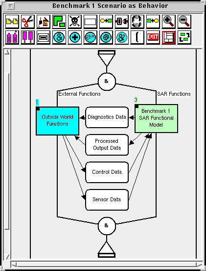
RDD-100 is used during this task to define the system functionality using an ALC graphical representation called a behavior diagram. The top level behavior diagram showing the
interaction of the SAR processor with its external environment is shown in Figure 4 - 3. The rectangular boxes represent functions, while the rectangular boxes with rounded corners indicate data items. The outside world (radar system) and the SAR processor functions appear on parallel branches in this figure since each can operate independently from each other. The flow of data between the SAR processor and its outside world is shown in this figure. The SAR processor receives control and sensor data from the outside world, while it sends output processed SAR and diagnostic data back to the external system. The black square in the upper corner of a box indicates there is a hierarchy of functions contained within that box. The top level system functionality is decomposed into lower level functions until the leaf level function can be allocated to a specific hardware or software item.
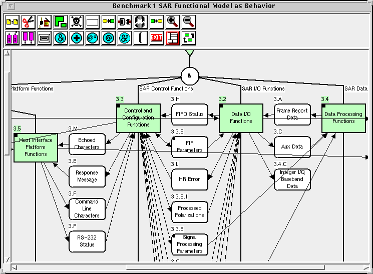
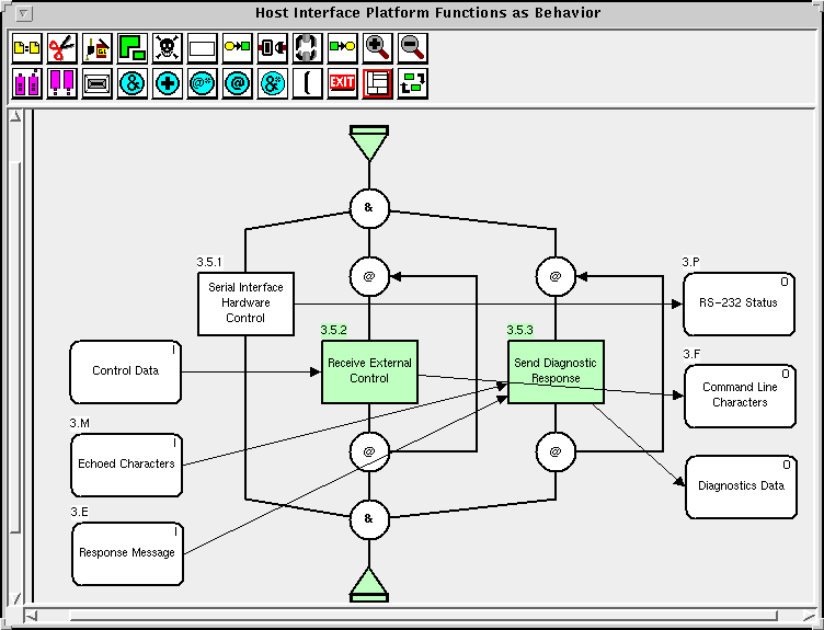
The next level of functional decomposition for the SAR processor is shown in Figure 4 - 4 (Only a portion of this diagram has been included in the figure due to its large size. A full view of this diagram is found in the SAR case study.) This diagram illustrates the top level functionality the processor and the data items passed among these functions. The functional decomposition for one of the top level functions (host interface platform functions) is shown in Figure 4 - 5. Note that both data and control flow are shown in this behavior graph. Data flow is shown from left-to-right, while control flow, illustrated by the loops in this diagram, is shown from top-to-bottom. The functional decomposition is used to fully characterize the set of functions, interfaces, control and data flow needed to meet system requirements.
Traceable links are established in RDD - 100 between the requirements and system functions to ensure that every requirement has been allocated to a function and that every function is directly attributed to a requirement. The links established in RDD - 100 for one of the originating requirement paragraphs are illustrated in Figure 4 - 6. The "specifies" relationship within the RDD - 100 schema is the relationship which links requirements to functions.
The use of the integrated tools which support the requirements and functional allocation, cost analysis and reliability tradeoffs is described within this
section. Emphasis is placed on illustrating how these three tools can be used cooperatively to perform tradeoffs that consider the entire life cycle.
PRL import file - An initial set of translation functions was developed and codified for signal processing applications on RASSP. These functions
define the mapping between 65 system engineering parameters and approximately the same number of PRICE parameters. The PRL import template
is typically generated once for a company and should address the complete product line and application domains. The baseline PRL import file
developed for RASSP is used in this example.
RDD-100 Output File - Attributes which characterize the system architecture, hardware, software and product life cycle must be populated in the
RDD-100 database prior to exporting the file needed for cost estimating. The types of attributes that must be entered into the RDD-100 database for
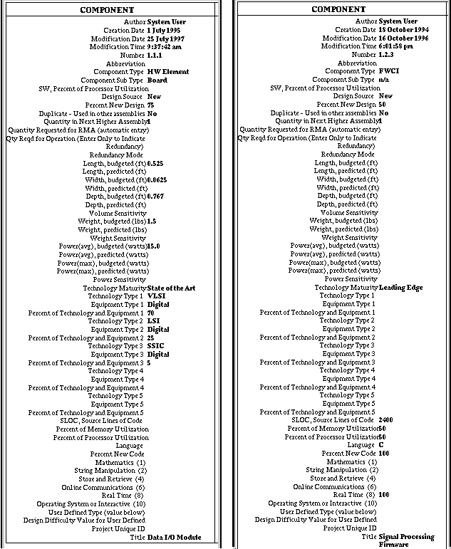
both a custom digital board (data i/o module) and software (signal processing firmware) are shown in Figure 4 - 9 . The data i/o module is a new,
custom board development requiring 75 percent new design. This board has a VME size and expected to weigh 1.5 pounds. The maturity of the
technology the board is built with is state-of-the-art technology with 70 percent of the board built with VLSI technology, 25 percent of LSI
technology and 5 percent of SSIC technology. The signal processing software is new code to be developed which requires 50 percent new design. The
technology maturity for the software development is leading edge. This software is written in the C programming language and is estimated to be
2400 lines of code. The software is characterized as real time software. Each system component must be characterized to this level of detail to generate
a cost estimate. The complete set of attributes for each component in the first candidate architecture is given in the appendix.
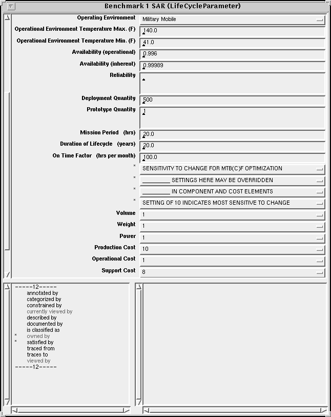
Attributes characterizing the system's life cycle must also be populated in the RDD-100 database. The life cycle attributes for this example are shown
in Figure 4 - 10. The operational environment, deployment quantity, mission period and duration of the life cycle are shown in this figure. The
sensitivity factors included at the bottom of Figure 4 - 10 are used in the RAM-ILS tool to optimize the physical configuration of the system to meet
reliability requirements. The production and support costs have been emphasized in this example.
A consistency report is run in RDD-100 which identifies whether a sufficient set of attributes have been populated to get a valid cost estimate. Once
the database is populated with the required parameters for costing purposes, an export report is run in RDD-100 that generates a file containing the
system engineering parameters in the correct format for cost estimating.
Cost Analyst File - The cost analyst file contains default PRICE parameters for each component in the system which are missing from translation of
the RDD-100 file. The parameters typically defined within the cost analyst file are prototype and production schedule, labor rates, escalation rates and
other financial factors that the PRICE tool needs. The information is entered within the cost analyst file on an element type basis. The cost analyst is
typically responsible for generating this file. The basic labor rates, escalation rates and financial factors included in the PRICE tool are used in this
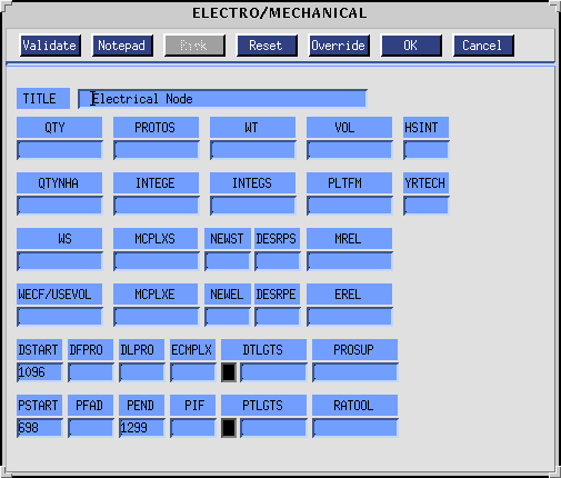
example. The only information specific for this example that is included within the cost analyst file is schedule information as shown in Figure 4 - 11.
This figure shows the default parameters for the electro-mechanical element type. The only information included for this element type is a 10/96
development start date, a 6/98 production start date and a 12/99 production end date.
Synchronization File - The synchronization file contains PRICE parameters for each component which supersede any parameter set from either the
translation of the RDD-100 file or cost analyst file. It is through the use of the synchronization file that the cost analyst can control the cost estimate
since any parameter within this file will take precedence over values set from any other source. The cost analyst is typically responsible for
generating this file. Information is entered in the synchronization file on a component name basis which enables each component to have its own
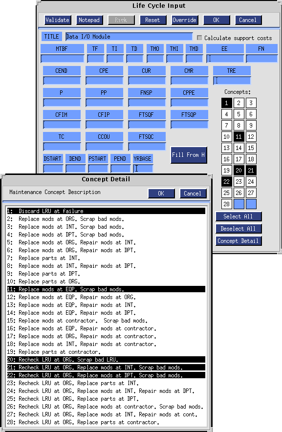
parameters within the synchronization file. The PRICE life cycle tool has various maintenance concepts that the tool can choose from in determining
the most cost effective concept . The maintenance concept is restricted to a subset of possible concepts in this example to illustrate the use of the
synchronization file. As shown in Figure 4 - 12, the maintenance concept for the Data I/O Module is limited to concepts 1, 11, 20, 21 and 22 (the
valid maintenance concepts are indicated by the black squares in this diagram). The definition for each of these concepts is included in the figure. The
PRICE toolset will select the most cost effective concept among these five potential maintenance concepts for this module regardless of any data
within either the RDD-100 file or cost analyst file.
Cost Estimate - The PRL import file, RDD-100 output file, cost analyst and synchronization files are used to populate the PRICE tool with all the
parametric cost estimating attributes needed to perform a cost estimate. The process to translate the system engineering parameters from the RDD-100
file to PRICE attributes and to apply both the cost analyst and synchronization file takes several minutes for this example. The equipment breakdown
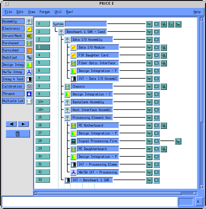
structure for the first candidate architecture after the data has been imported into the PRICE toolset is shown in Figure 4 - 13. This equipment
breakdown structure is identical to the physical equipment tree established in RDD-100. The tree icons in this figure represent assemblies which
contain lower level components. Note that the backplane and host interface assemblies have been collapsed in this figure to reduce its overall size.
The lightning bolt icon represent custom digital boards, while the dollar icons are COTS items. The workstation icon represents a software
component. Note that elements of both hardware and software are contained within this single equipment tree. Design integration, hardware/software
integration, and integration and test elements are added in the appropriate places to the PRICE equipment tree during the translation process even
though these elements are not included within the RDD-100 database. The costs for these integration elements are included as a part of the assembly
level costs when exporting the cost data back to RDD-100.
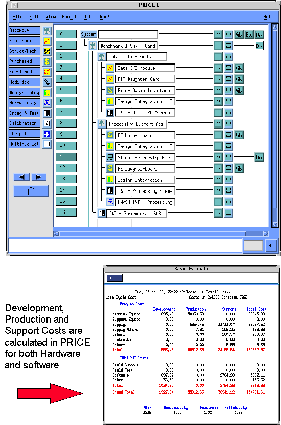
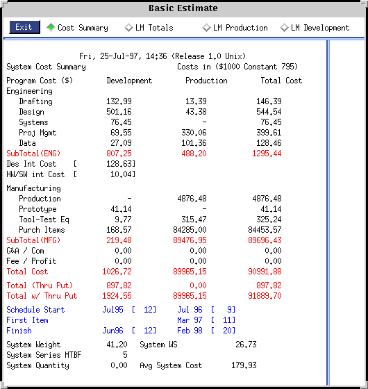
The development and production cost estimates from the PRICE tool for the first candidate architecture are shown in Figure 4 - 14. The first column in
this figure shows the development costs and the second column depicts the production costs. The engineering costs are in the top half of the cost
summary, while the manufacturing costs are in the bottom half. The development costs for the first candidate architecture is $1.9M and the
production costs for 500 systems is $90M. The average system cost is $179.9K.
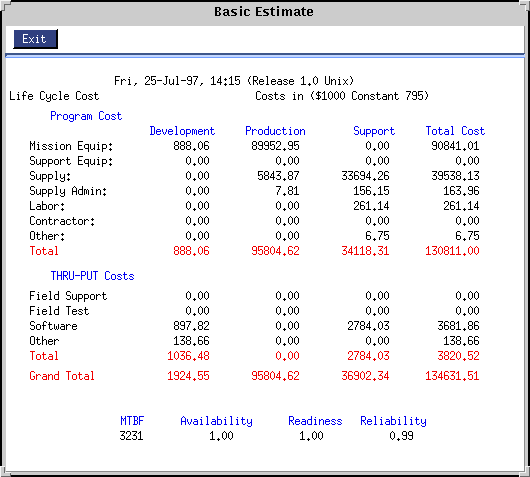
The life cycle cost estimates from the PRICE tool for the first candidate architecture are shown in Figure 4 - 15. The first column in this figure shows
the development costs, the second column gives the production costs for the 500 systems and initial spares, and the third column shows the support
costs over the twenty year life cycle. The total life cycle costs for this architecture is $134.6M.
Export of Costs to RDD-100 - The development, production and support cost estimates calculated by the PRICE toolset are back annotated in the
RDD-100 database. This back annotation is performed by exporting the cost data out of the PRICE tool into a file with the standard rdt format which
RDD-100 uses. This file is generated by executing a PRL export script within the PRICE toolset. This file is then imported into RDD-100 using the
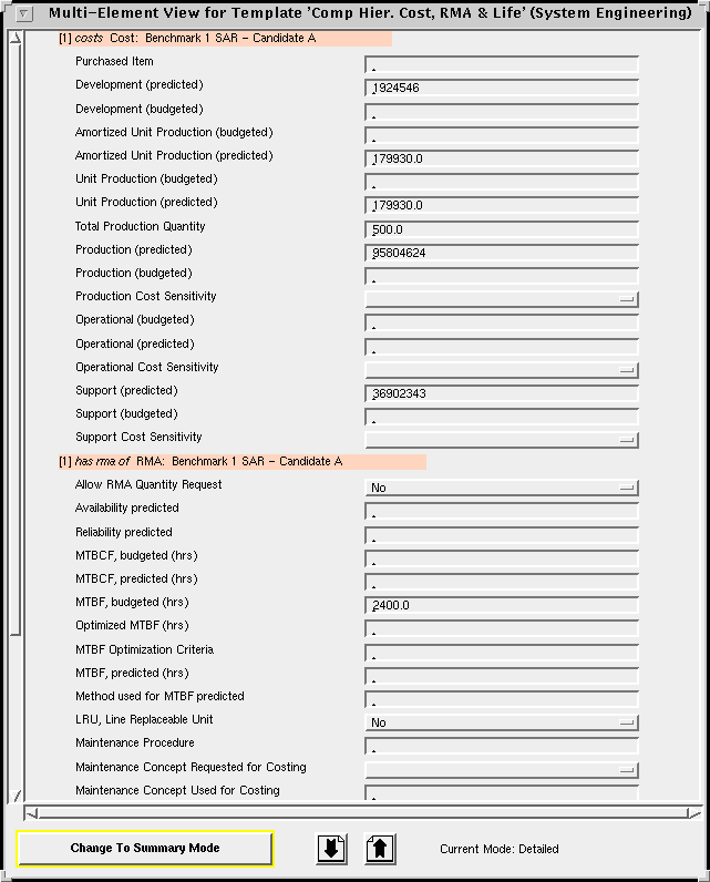
standard import facility. An RDD-100 view of the cost and reliability data for the SAR system for the first candidate architecture is shown in Figure
4 - 16. The costs in this figure were calculated in the PRICE tool. The reliability data in this figure is empty, as this analysis will be performed in the
next section.
Attributes which characterize the system architecture and the hardware components must be populated in the RDD-100 database prior to exporting the
file needed for reliability assessment. Most of these attributes are the same attributes needed to generate the cost estimate for the PRICE tool. The
attributes used to characterize the data i/o module have been previously shown in Figure 4 - 9. Redundancy parameters are included in this set of
parameters which are used within the RAM-ILS tool for the reliability assessment. For this example, there is no redundancy included in the initial
system architecture. Tradeoffs are performed within the RAM-ILS tool in this example to determine how the system architecture can be changed in a
cost effective way to meet system reliability requirements.
A reliability assessment can be performed using the RAM-ILS based upon previous designs, similar to designs or from the allocated failure rate
budget. The reliability assessment in this example is based upon the allocated failure rate budget as the focus of this example is showing how the
integrated tools can be used early in the design process when detailed design data is not available. The systems engineer allocates the system level
mean time between critical failures (MTBCF) to the system components within the RDD-100 tool. The system engineer performs this allocation
based upon available component data, interactions with reliability engineers and his judgment based on past experience. Parameters specific to
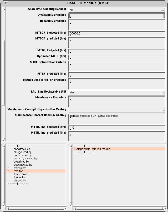
reliability and maintainability are entered in the RMA entity type for each component. The RMA entity for the data i/o module is shown in Figure
4-17. A MTBCF of 30,000 hours has been allocated to the data i/o module. The system engineer also indicates in this entity type whether the
component can be considered for redundancy when performing a system architecture optimization within the RAM-ILS tool. Redundancy is not
allowed for the data i/o module in this example (attribute name is Allow RMA Quantity Request within the RDD-100 schema). Note that the
maintenance concept which the PRICE toolset selected for its life cycle support optimization has been back annotated in the RDD-100 database. In
addition, a mean time to repair (MTTR) and an indication whether this component is a line replaceable unit have been indicated in Figure 4 - 17. The
complete set of attributes for each component in this example is given in the Appendix.
The operational environment for the system must be defined prior to performing a reliability assessment. This environment is specified within the
Life Cycle Parameter entity type in RDD-100 and the life cycle attributes for this example were previously shown in Figure 4 - 10 as many of these
parameters are needed in the PRICE tool to calculate support costs.
Optimizations are performed within the RAM-ILS toolset to determine the most effective architecture which satisfies the system level reliability
requirements. The system configuration can be optimized relative to size, weight, power, cost or a combination of these factors. The user must
indicate the importance of these metrics on a relative basis either at the component or system level. The sensitivity factors are defined at the system
level and emphasize production and support costs for this example as shown in Figure 4 - 10.
A consistency report is run in RDD-100 which identifies whether a sufficient set of attributes have been populated to get a valid reliability
assessment. Once the database is populated with sufficient parameters, an export report is run in RDD-100 that generates a file containing the system
engineering parameters in the correct format for reliability assessment. This file is then imported into the RAM-ILS toolset which establishes the
system architecture and the pertinent parameters needed to perform a reliability estimate. A reliability assessment based upon the equipment
configuration and allocated budgets is made within the predictor portion of the RAM-ILS toolset. An output report containing the reliability
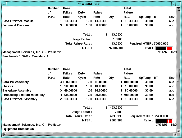
assessment at the system level from the RAM-ILS tool for this example is shown in Figure 4 - 18. The mean time to critical failure (MTBCF) for the
first candidate architecture is calculated as 2068 hours. This system configuration did not meet the required 2400 hour system-level MTBCF. As a
result, the system configuration must be changed to meet the reliability requirement.
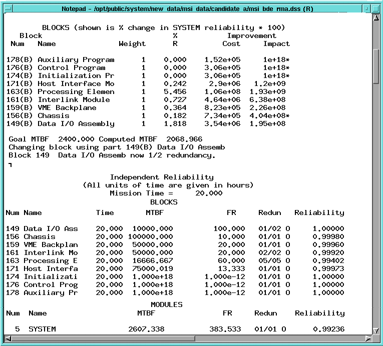
The block diagram evaluator (BDE) portion off the RAM-ILS toolset is used to optimize the physical architecture when requirements are not met.
This optimization is performed by determining both the overall improvement in the system-level MTBF and the associated cost for adding redundancy
for each hardware component in the system. The output of BDE for the first candidate architecture is shown in Figure 4 - 19. The first column in this
output report shows the improvement in the system-level reliability when an additional redundant unit is added for a particular component. The second
column shows the aggregate cost of this additional redundant unit which is calculated from the component's physical parameters and sensitivity
factors. The third column in this report shows the impact of adding redundancy for this particular component which is calculated by dividing the cost
of the redundancy by the overall improvement. The component with the smallest number in the third column is the most cost effective place to
initially add redundancy to improve the system-level reliability. The data I/O assembly is the most cost effective component to add redundancy in this
example. The RAM-ILS tool then determines the overall system-level MTBCF when the most cost effective redundant component is added to the
system architecture. This procedure iterates until the system requirements are met. For this example, the MTBCF improves to 2607 hours and meets
the overall requirements when a redundant data I/O assembly is added to the system architecture.
The results of the reliability assessment calculated by the RAM-ILS toolset are back annotated in the RDD-100 database. This back annotation is
performed by exporting the reliability data out of the RAM-ILS tool into a file with the standard rdt format which RDD-100 uses. This file is
generated automatically within the RAM-ILS toolset after the reliability calculations are made. This file is then imported into RDD-100 using the
standard import facility. The reliability results that are back annotated into the RDD-100 database are for the baseline system configuration sent to the
RAM-ILS tool. A critical issue is generated in the RDD-100 database when the allocated reliability budgets are not met. All optimizations results
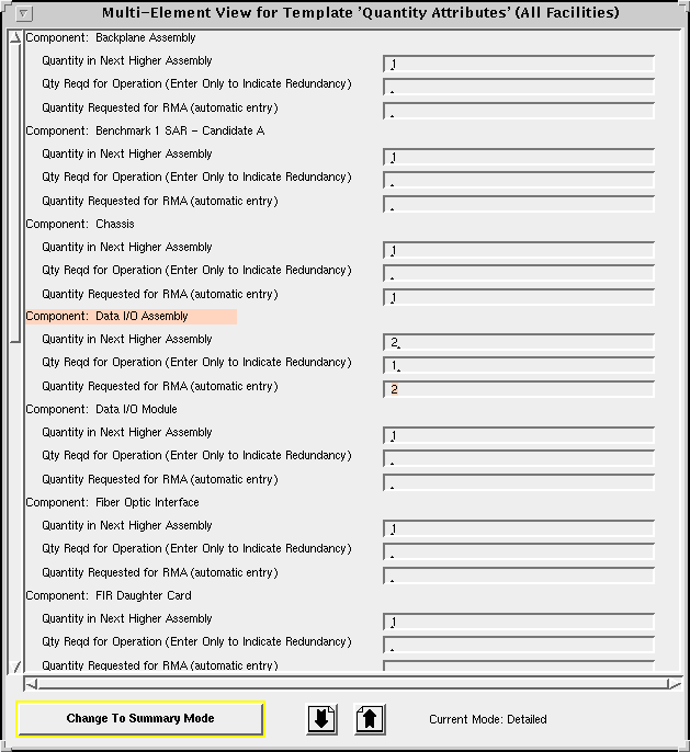
obtained using the RAM-ILS toolset are back annotated in the RDD-100 database as a suggestion for change, as shown in Figure 4 - 20 for this
example. The system engineer must determine whether to accept the redundancy recommendation or make other changes to meet the requirements. For
this example, redundancy at the data i/o assembly is acceptable and the system architecture must be changed by the systems engineer in the RDD-100
database to reflect this redundancy.
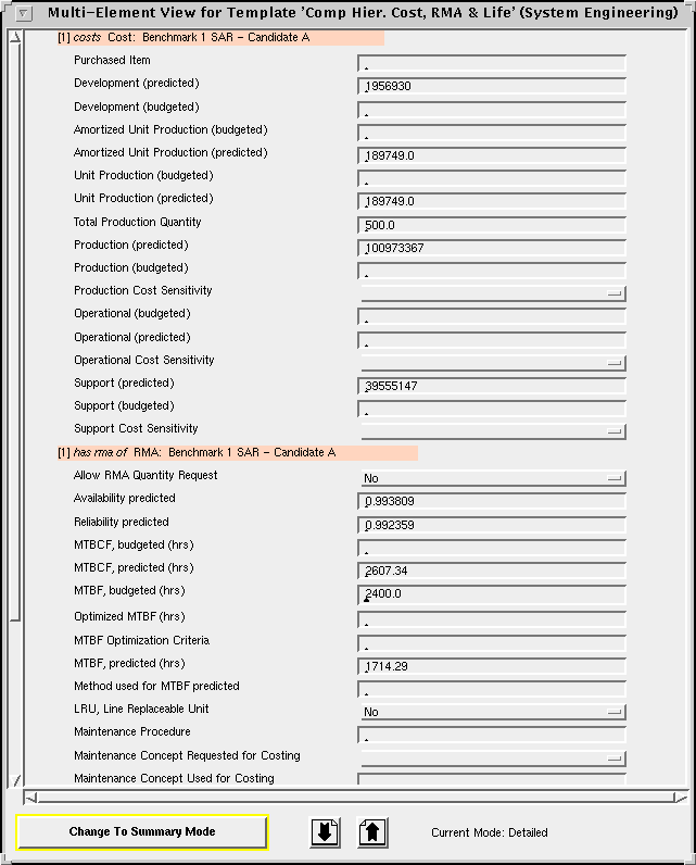
An updated reliability assessment and cost estimate is needed whenever the physical configuration of the system is changed. Thus, the processes used
to generate both a cost estimate and reliability assessment are repeated when the data i/o assembly redundancy is added to the system architecture in
this example. The resulting costs and reliability estimate for this system with redundancy are summarized in Figure 4 - 21. The development costs
increased by $30K, the per unit production costs have increased by $10K and the support costs have increased by $2.6M when the redundant data i/o
assembly is included in the system architecture for the first candidate.
This example illustrates how important it is to perform cost and reliability trade-offs early in the design cycle. These tradeoffs must consider the
entire life cycle as opposed to the costs for a particular phase of the program. As can be seen from this example, a slight increase in costs during the
development phase results in significant life cycle cost savings.
First Candidate Second Candidate Development Costs $ 2.0M $ 2.1M Production Costs $ 101.0M $ 81.1M Unit Production Costs $ 190K $ 151K Support Costs $ 39.6M $ 29.8M Total Life Cycle Costs $ 142.5M $ 113.0M MTBCF 2607 hours 3297 hours MTBF 1714 hours 3297 hours
As shown in the SAR example, it is possible to select the wrong architecture if the decision is only based upon the development costs. The life cycle
costs in this example were reduced by over 20 percent just by understanding these costs early in the development phase. This information is critical in
achieving the RASSP goal of reducing life cycle costs by a factor of four. Although the RASSP concurrent system engineering environment has
been developed to work well in the signal processing domain, many of these concepts can be extended for higher level systems.
4.0 Technical Description
4.1 SAR Benchmark Overview
4.2 Requirements Analysis
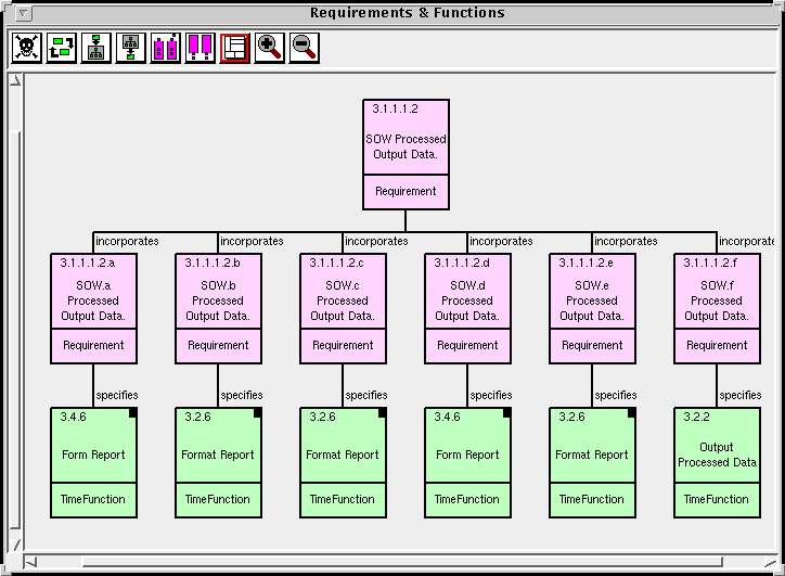
RDD-100 is used to support the requirements analysis task for the SAR benchmark. The system level requirements for the SAR processor are contained within a technical description document. The text for each requirement paragraph of this document is initially parsed into its own requirement within RDD-100. Each requirement paragraph is then refined and decomposed into lower level requirements within RDD-100. Each requirement must be decomposed to a single testable unit so that it can be verified during system acceptance testing. An illustration of the requirements decomposition is shown in Figure 4 - 2 . A graphical representation of one requirement paragraph decomposed into lower level requirements within RDD-100 is shown in this figure. A naming convention which incorporates SOW as part of the requirement name is used so that the source requirements are readily apparent within the database. This top level requirement is decomposed into six lower level requirements as the initial requirement paragraph within the technical description document actually contains multiple requirements. The "incorporates" relationship within the RDD-100 schema is the relationship which links a parent requirement to a child requirement. This requirements decomposition is used to identify and resolve any ambiguous or missing requirements with the customer. The decomposed and refined set of requirements is used to generate the specification for the signal processor.

4.3 Functional Decomposition
A functional decomposition of the SAR processor is performed after the initial set of requirements are well understood. This decomposition is performed by defining the set of
functions, interfaces, control and data flow needed to satisfy the system requirements. The initial functional decomposition is performed without the notion of the physical architecture. However, this process is performed concurrently with the system partitioning task, as elements of the physical architecture impact the physical decomposition. Behavioral simulations (see the Token-Based Performance Modeling application note) of the system are performed during functional decomposition using other complimentary tools/languages to ensure that all system requirements are met.
4.4 System Partitioning
System level tradeoffs are performed during the system partitioning task to determine the most effective set of subsystems needed to satisfy the
requirements. All aspects of the system's life cycle should be considered when performing these tradeoffs. The system partitioning task is performed
concurrently with functional decomposition since the selection of subsystems does impact the functional decomposition.
4.4.1 Requirements & Functional Allocation
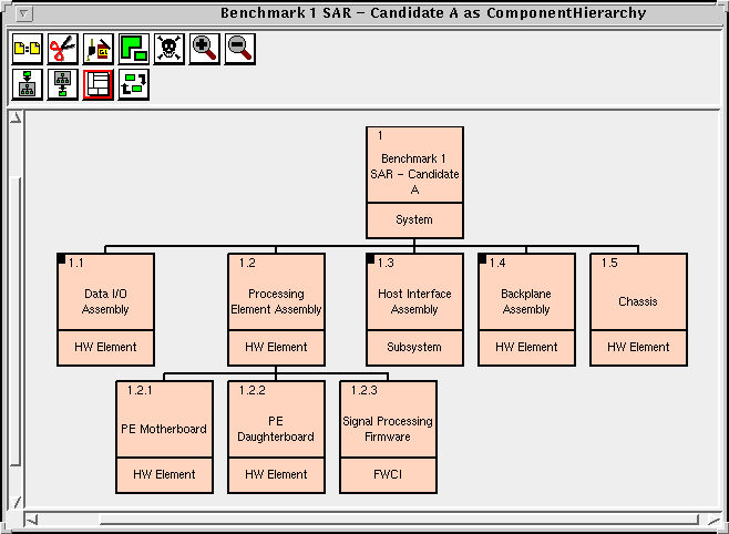
The third view of a system within RDD-100 is the physical view. The equipment tree for the first architecture (mature signal processor) in this
example is shown in Figure 4 - 7 . Each of the blocks in this figure represents either a hardware or software component in the system. Traceable links
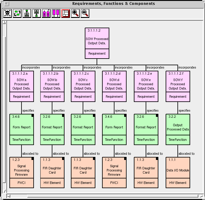
are established in RDD-100 between the system functions and components to ensure that every function has been allocated to a component and that
every component is directly attributed to a function. The links established in RDD-100 for one of the originating requirement paragraphs are
illustrated in Figure 4 - 8 . The "allocated to" relationship within the RDD-100 schema is the relationship which links functions to components. The
full set of military specifications can be generated from the information within the RDD-100 database.
4.4.2 Cost Analysis
The RDD-100 schema has been enhanced on RASSP so engineers can easily get a cost estimate to support system level tradeoffs. Four different files
are needed to generate a cost estimate: a PRICE Rule Language (PRL) import file which contains the translation functions needed to convert system
engineering parameters into cost estimating attributes, an output file from RDD-100 which contains the system engineering parameters for the
system being costed, a cost analysis file which contains default cost estimating parameters and a synchronization file which contains parameter values
which supersede the values obtained from translation of the system engineering parameters. Each of the files used to generate the cost estimate for
this example are described below.
4.4.3 Reliability Assessment
A preliminary architecture has been defined and an initial cost estimate calculated for the first candidate system. A reliability assessment of this
system is made next to ensure that all requirements are met. The RDD-100 schema has been extended on the RASSP program to support this
reliability assessment. The only external data that the RAM-ILS toolset needs to perform a reliability assessment is contained within the file
generated within RDD-100. This file contains the complete system architecture, physical attributes of the system components, allocated reliability
budgets, parameters characterizing the operational environment, sensitivity parameters and cost data. Each of these elements is described in more detail
below for the SAR example.
4.4 System Cost And Reliability Assessment
In the previous section, a cost estimate and reliability assessment were made for the first candidate architecture. The same procedure is used to
determine the cost and reliability for the second candidate architecture. The second architecture did not require redundancy as the baseline system met
the system reliability requirements. The cost and reliability results for both architectures are summarized in Table 4-1. The development costs are
$100K more expensive for the second architecture. However, the per unit production costs are $39K cheaper for the second architecture and the
support costs are also approximately $10M cheaper. The total life cycle costs for the second candidate architecture is almost $30M cheaper than the
first architecture. In addition, the reliability of the second candidate architecture is superior than the first system.
Architecture
Architecture
4.5 Summary
The ATL RASSP team have developed a concurrent engineering environment consisting of three existing computer tools (RDD-100, PRICE cost
estimating tools and RAM-ILS). This system design environment quickly provides more detailed and accurate information to the integrated product
team and enables them to make better informed decisions early in the development process. Since these early decisions have the largest impact on the
overall life cycle costs of a system, it is important that these decisions be based on all life cycle costs and not just the cost of initial development.
![]()
![]()
![]()
![]()
Next: 5 References
Up: Appnotes Index
Previous:3 Technical Description