Adapting Differential Fault Simulation For VHDL Implementation
Alireza Khalafi and Zainalabedin Navabi
Electrical and Computer Engineering Department
Faculty of Engineering, Campus No. 2, University of Tehran
14399, Tehran IRAN
navabi@khorshid.ut.ac.ir
ABSTRACT
To reduce simulation events, a differential fault simulator simulates all faulty circuits for the same test input before applying the next test vector to the circuit. Activities occur in limited parts of a gate level circuit between application of faults for the same input vector. Adapting this fault simulation technique to the programming environment of VHDL and its use in fault simulation of sequential circuits will be presented in this paper. Modeling gate level lines and components in VHDL will be presented.
1. Introduction
Fault simulation is a CPU intensive process due to the fact that a circuit has to be simulated for thousands of faults and thousands of test vectors. In most fault simulators, faulty circuit models are generated for every possible circuit fault and these circuits are all simulated for all the test vectors. Changing a test vector at the primary inputs of a faulty circuit causes events to propagate throughout a circuit which results in simulation activities. To reduce simulation time, the order of applying test vectors can be chosen such that two consecutive tests cause minimal activities in the circuit. This method, however, can only be used for fault simulation of combinational circuits in which the order of the tests is not significant.
A differential fault simulator reverses the order of test application and fault insertion. A test applied to a faulty circuit will remain at the primary inputs until the circuit is simulated for all possible faults. Simulation activities can be minimized by choosing the ordering of inserting faults (or applying faults, as it more corresponds to the way they are done here) such that two consecutive faults will be affecting the same area of the circuit under test. Because the ordering of the test vectors remains intact, sequential circuit fault simulation can benefit from ordering of faults in a differential fault simulation. In fault simulation of sequential circuits, memory state of the circuit must be saved between application of faults.
Differential fault simulation has been implemented in VHDL by writing gate, line and flip-flop VHDL models. A VHDL testbench provides test vectors and faults to the circuit model and is responsible for starting and stopping the simulation of the circuit for the inserted faults and applied tests. Reporting faults and fault coverage will also be done by the testbench. Data structures in the flip-flop models and the testbench are responsible for keeping track of circuit states and detected faults.
This paper presents an overview of the differential fault simulation, and its adaptation for implementation in VHDL programming environment. Details of VHDL component and circuit analyzer descriptions will be presented. Flip-flops models play an important role in the implementation of differential fault simulation. VHDL implementation of flip-lop models will be emphasized in this paper. Example runs from ISCAS89 benchmarks are provided in the last section of the paper. These results are compared with those of a concurrent fault simulator.
2. Differential Fault Simulation
The simplest technique for fault simulation is serial fault simulation. In this method, a fault will be inserted into the circuit and test vectors are applied one at a time. The main disadvantage of this fault simulation method is the time it takes for running simulations or all test vectors as many times as there are faults in the circuit. This method does not require any special software and a standard gate level simulator can be used for this purpose. Other approaches such as concurrent or parallel fault simulation are used for a better performance. The success of a concurrent fault simulator lies in the fact that only the difference between the good model of the circuit and faulty circuits are simulated. Since the difference between a good and a faulty circuit is only at the site of a fault, the values of the majority of the signals in the two circuits remain the same. Simulation speed is improved by simulating only those parts of the circuit that are different from the good circuit. Therefore, instead of recording the circuit status of all the bad machines, a concurrent fault simulator records the differences between faulty circuits and the good machine. Concurrent fault simulation is efficient but it requires a dedicated simulation program.
for every test vector, Vi,
{ /* compute good machine circuit status */
if (Vi is the first vector)
{ Initialize circuit status; }
else
{ Remove the previously injected fault;
Recover current states;}
Set Vi pattern at the primary inputs;
Perform event-driven simulation;
/* compute faulty machine circuit status */
for every undetected faulty machine, Bj,
{Remove the previous injected fault;
Recover current states;
Inject current fault;
Perform event driven simulation;
if the fault is detected
Drop the fault;}
}
Figure 1. Differential Fault Simulation Algorithm
To reduce the memory requirement of concurrent fault simulators and dynamic fault list manipulations that is necessary for sequential circuits, Cheng and Yu have presented differential fault simulation as a new method of fault simulation. The main difference between this method and previous approaches is the order in which faults and test vectors are applied. In conventional methods a fault is initially inserted into the circuit and test vectors are applied to find the response of the various circuits to these tests. Simulation ends when all faulty circuits have been tested for all test vectors. In the differential fault simulation, a test vector is applied to the circuit and all undetected faults will be inserted in the circuit one after another. This will result in much less activity in the circuit, use of little overhead memory, and can be implemented by VHDL models using the standard VHDL simulator. The general outline of this approach, which we shall refer to as DSIM, is shown in Figure 1.
In this algorithm, a test vector is applied to the circuit and the good machine will be simulated for that test. After simulation of the good machine, simulation will be done for every undetected fault with the same test vector. This is done by applying a test and injecting an undetected fault to the circuit model and performing the simulation. Simulation results will be compared with that of the fault-free circuit. The injected fault is detected if primary outputs of the faulty circuit are different than those of the good circuit. In this case the fault will be removed from fault list, otherwise the memory status of the faulty circuit will be saved for fault simulation of the next test vector. This is illustrated in Figure 2. The process of applying tests and examination of faulty circuits continues until a satisfactory fault coverage has been reached or there are no more test vectors.
Referring to Figure 2, in the first time frame, the output values of all circuit memory elements are X and all the good and bad machines will be simulated with the applied test vector (V1). Since simulation of the next time frame must be the continuation of the present time frame, faulty circuits save their current status to be restored in the next time frame (f1,1, f2,1, and f3,1 states of f1, f2, and f3 faulty circuits are saved in the first time frame). To keep the current status of a circuit, it is sufficient to store the input value of all circuit flip-flops. This is achieved by flip-flops having internal storage capability which has been implemented as a dynamic list to reduce memory requirements.
In the next time frame, the next test vector (V2) will be applied to the circuit and the faults will be injected to the circuit. For every faulty circuit the flip-flop output values will be retrieved so that the circuit returns to its correct status for the simulation to continue from this point on. Also in each simulation step, if the inserted fault is detected, it will be removed from fault list and its corresponding allocated memory in flip-flop internal data structure will be freed. An example of this case is fault f2 in Figure 2 which has been detected in the second time frame and its state (f2,1) removed. The fault is detected because its effect propagates to the circuit primary outputs.
It is worth noting that unlike concurrent fault simulation that requires the value difference information on every node, this method only requires the value difference information on the flip-flops. This results in a substantial less memory requirement for the differential fault simulator.
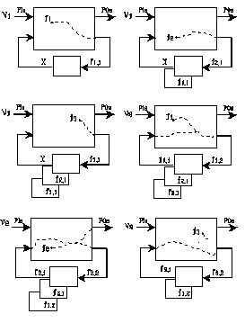
Figure 2. Fault Simulation Steps
3. DSIM VHDL Implementation
Differential fault simulation has been implemented by modeling gates and wires in VHDL and running VHDL simulation for performing fault simulation. The VHDL implementation consists of a circuit analyzer and an interconnection of gates and wires. The circuit analyzer is responsible for construction of a fault list, reading test vectors from an input file and simulation of the circuit for all undetected faults. After simulating with each test vector, the output response will be analyzed and detected faults will be removed from fault list. This process will be done for all test vectors and the final fault coverage will be reported by the circuit analyzer.
A block diagram of our VHDL differential fault simulation environment is shown in Figure 3. The primary inputs and outputs of the sequential circuit are connected to the circuit analyzer which applies test vectors to the circuit and analyzes the output response. The fault list is also implemented as a dynamic linked list that facilitates removal of detected faults. Two global signals are used for injecting faults to the circuit. The first signal represents the id number of the line to be faulted and the second represents the fault type, i.e. stuck at 0 or stuck at 1. The sections that follow describe modeling for gates, wires, flip-flops, and the circuit analyzer in VHDL.
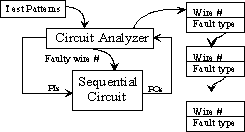
Figure 3. Fault Simulation Testbench
3.1. Gates and Wires
Most digital circuits can be considered as a collection of gates that are connected by signal lines. Since the main functionality of the circuit is based on the functionality of its gates, the usual way for modeling a circuit in VHDL is writing a model for each gate and connecting them by signals. These signals have no special task except carrying values from one place to another. Although this is an accepted way for describing circuit structures, for our fault simulation, we found it more convenient to model lines as components and gates as resolution functions. In other words, instead of considering the circuit as a set of gates that are connected by lines, we have considered it as an interconnection of lines that are joined by gates. Figure 4 shows these two gate level structures.
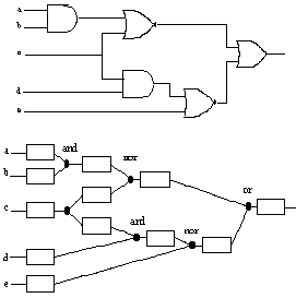
Figure 4. Gate Level Description Alternatives
In our approach, lines are assumed to be components with a special functionality appropriate for fault simulation. These lines are connected by a series of resolved signals which represent various logic gates.
The first and most important advantage of this modeling method is that it allows gates with any number of inputs. In the conventional modeling style, several models must be developed for the same logical function with different number of inputs. Using a resolution function for gate models, allows multiple signals to be connected to the same function.
ENTITY wire is
GENERIC (id_num : NATURAL);
PORT (input : IN qit; output : OUT qit);
END wire;
ARCHITECTURE behavioral OF wire IS
BEGIN
-- faulty_wire and fault_type are global signals
PROCESS (inputs, faulty_wire)
BEGIN
IF(id_num /= faulty_wire) THEN
output <= input;
ELSIF (fault_type = s_a_0) THEN
output <= 0';
ELSE
output <= 1';
END IF;
END PROCESS;
END behavioral;
Figure 5. Wire VHDL Code
The second advantage of our approach is the ease of fault insertion. In a gate level fault simulator the most widely used fault model is stuck at fault. This fault model assumes that the gates are fault free and only the interconnecting signal lines may be affected by a fault. Therefore, modeling lines instead of gates can make fault insertion more convenient. VHDL code of a signal line is shown in Figure 5. Type qit is defined as a four value logic type with 0', 1', Z' and X' enumeration elements.
As seen in this description, when there is no fault on a line, it simply propagates values from one end of the line to its other end (output). In the presence of a fault, the signal line will have a fixed 0 or 1 value depending on the fault type. Presence or absence of a fault is determined by comparing a line id number with faulty_line global signal. Each line has a unique id number that distinguishes it from other lines. Fault on a line is inserted by assigning its id number to the fault specification global signals.
SIGNAL nand1 : nand_gate;
SIGNAL input1, input2, output1 : primary_io;
w1 : a_wire GENERIC MAP (1)
PORT MAP (input1, nand1);
w2 : a_wire GENERIC MAP (2)
PORT MAP (input2, nand1);
w3 : a_wire GENERIC MAP (3)
PORT MAP (nand1, output1);
Figure 6. Representing a 2-Input NAND Gate
Logic gates are implemented by resolution functions. The resolution function of a NAND gate will simply return the NANDed value of all signals driving it. This can be taught of as a gate that changes its number of inputs as required by the driving lines. Figure 6 shows the VHDL code for implementing a two input NAND gate. Two lines are used for gate inputs and one line for the gate output.
3.2. Flip-flop Modeling
In a sequential circuit, flip-flops transfer data between subsequent time frames. In our fault simulator, a test vector is applied during a time frame and flip-flop input values in good and faulty machines may be different at the same time frame. Thus, as shown in Figure 2, to set the outputs of flip-flops to the correct value at the next time frame, it is necessary to save their current input values. In circuits with many flip-flops, saving all flip-flop values for all faults may require a large amount of memory. On the other hand, in most circuits there are only a small subset of flip-flops with different values in good and faulty machines. Therefore, to reduces memory requirements and dynamic list manipulations, we only save those input values of faulty machine flip-flops that are different from those of the good machine.
The pseudo code of a flip-flop model is shown in Figure 7. A flip-flop model has its own fault list in which it keeps the value differences for those circuit faults that propagate to that specific flip-flop. A linked list is used to store flip-flop values of the good and faulty machines. After simulation of the good machine, the input value of the flip-flop is stored for comparison with bad machines. In simulation of the faulty circuits, if the fault that is being simulated appears in the current list of a flip-flop, it means that the fault has propagated to that flip-flop and the output value of the flip-flop in the faulty machine is different from that of a good machine. In this case, the output must be set to the stored value. Otherwise the output will be set to the good machine output value.
ENTITY flipflop IS
PORT (input : IN qit; output : OUT qit);
END flipflop;
ARCHITECTURE behavioral OF flipflop IS
BEGIN
PROCESS . . .
BEGIN
WAIT UNTIL new fault simulation run;
IF (good machine is being simulated) THEN
good_value <= input;
ELSE
IF current fault exists in my fault list THEN
output <= faulty value;
ELSE
output <= good_value;
END IF;
WAIT FOR combinational part simulation;
IF input /= good_value THEN
IF current fault not exist in fault list THEN
create a new entry in fault list;
save input value;
ELSE
replace saved value with input value;
END IF;
ELSE
IF current fault exists in fault list THEN
remove this entry from fault list;
END IF;
END IF;
IF fault is detected THEN
IF current fault is in my fault list THEN
remove this entry from fault list;
END IF;
END IF;
END IF;
END PROCESS;
END behavioral;
Figure 7. Pseudo code of a flip-flop model
After simulation of a faulty circuit, if the fault is detected or if the input of the flip-flop is the same as that of the good machine, there is no need to store this value and it will be removed from the internal flip-flop list to reduce memory requirements. On the other hand, if the input value of the flip-flop is different from that of the good machine, it will be saved to be used in the next time frame (when the next primary input test vector is applied).
The list containing the flip-flop value differences are kept internal to each flip-flop. This is a linked list and grows hen faults propagate to flip-flops, and shrinks when faults are detected, or good circuit values reach flip-flops of a faulty circuit. This list has been implemented as an ACCESS type shared variable local to flip-flop models.
ENTITY circuit_analyzer IS
GENERIC (total_wires : NATURAL);
PORT (inputs : OUT qit_vector;
outputs : IN qit_veqtor);
END circuit_analyzer;
ARCHITECTURE behav OF circuit_analyzer IS
BEGIN
PROCESS . . .
BEGIN
read_faultlist();
WHILE NOT ENDFILE (test_patterns) LOOP
READ (test_vector);
-- Simulate good circuit first
inputs <= test_vector;
fault_type <= no_fault;
WAIT FOR simulation of circuit;
good_outputs := outputs;
WHILE faults exist in fault list LOOP
inject fault;
WAIT FOR simulation of the circuit;
IF output /= good_outputs THEN
fault is detected, remove it;
ELSE
fault is still not detected;
END IF;
END LOOP;
END LOOP;
calculate fault coverage and generate report;
WAIT;
END PROCESS;
END behav;
Figure 8. Circuit Analyzer Pseudo Code
3.3. Circuit Analyzer
In our fault simulator, applying test vectors, analyzing output response, removing detected faults from fault list and reporting the final fault coverage are done by a component called circuit analyzer. The pseudo code of this component is shown in Figure 8. The architecture of this component uses a single process statement. In this process, the fault list that may be the output of a fault collapsing program is initially read from an external input file. Then for each undetected fault, the corresponding bad machine will be simulated. At each time frame, if the value of any primary output signal of the bad machine is different from that of the good machine, the fault is detected and will be removed from fault list. Otherwise it will remain in the fault list to be simulated with other test vectors. After simulation of all test vectors the fault coverage and undetected faults will be reported.
4. Results
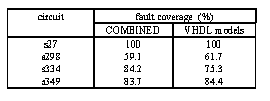
Table 1 shows the results of fault simulation for several circuits of the ISCAS89 sequential benchmarks. The circuits are simulated with random test vectors and the results are compared with those of the COMBINED[7] fault simulator. This table shows that the results are comparable with those of a concurrent fault simulator. The simulation time, however, is substantially more with VHDL models using a commercial VHDL simulator.
5. Conclusions
This paper presented VHDL models for fault simulation of synchronous sequential circuits. These models are based on a novel method that has better performance than conventional methods. Obviously this performance improvement does not cause VHDL models to simulate as efficient as conventional fault simulators. However, the goal here has been to illustrate that a standard VHDL simulator can be used for fault simulation and adapt a technique for this purpose that will minimize the performance penalty. The use of a VHDL netlist that can be used for simulation, test generation and fault simulation in an integrated VHDL based design environment, and the use of the same VHDL simulation program for all such applications is the main intention of this and other works on VHDL testing by our research group.
Table 1. Fault Simulation Results
For this scheme of VHDL fault simulation to be of practical use, standard file formats for test vectors and fault lists must be developed for better test data exchange between various applications. A parallel fault simulation based on this scheme will greatly improve the simulation speed. Also, to improve the simulation speed, faults should be ordered such that succeeding faults injected in the circuit under test are in the same area of the circuit. This way circuit activities between application of one fault to the next will be minimized.
References
[1] T. M. Niermann, Wu-Tung Cheng, and Janak H. Patel, "PROOFS: A Fast, Memory-Efficient Sequential Circuit Fault Simulator," in IEEE Trans. Computer-Aided Design, Vol. 2, No 2, pp. 198-207, Feb. 1992.
[2] H. K. Lee and D. S. Ha, "New Methods of Improving Parallel Fault Simulation in Synchronous Sequential Circuits," in Proc. Int. Conf. on Computer Aided Design, pp. 10-17, Oct., 1993.
[3] E. G. Ulrich and T. G. Baker, "Concurrent Simulation of Nearly Identical Digital Networks," Computer, Vol. 7, No. 4, pp. 39-44, April, 1974.
[4] W. T. Cheng and M. L.Yu, "Differential fault simulation -- A new method using minimal memory," in Proc. 26th Design Automation Conference., pp. 424-428, June, 1989.
[5] Z. Navabi, VHDL: Analysis and Modeling of Digital Systems, McGraw-Hill Publishing, New York, 1993.
[6] Z. Navabi, N. Cooray and R. Liyanage, "Using VHDL in Parallel Fault Simulation," in Proc. scs. Int. Conf. on simulation in Engineering Education, January 17-20, 1993, Vol. C-25, pp. 198-203
[7] M. Mojtahedi and W. Geisselhardt, "New Methods for Parallel Pattern Fast Fault Simulation for Synchronous Sequential Circuits," in Proc. Int. Conf. in Computer Aided Design, pp. 2-5, 1993.
[8] F. Berglez, D. Bryan, and K. Kozminski, "Combinational Profiles of Sequential Benchmark Circuits," in Proc. Int. Symp. on Circuits and Systems, May 1989, pp. 1929-1934.